 Figure
1 Spherical
polar coordinates, related to Cartesian coordinates
Figure
1 Spherical
polar coordinates, related to Cartesian coordinates Structure of the Periodic Table
The Correlation of Atomic Spectral Behaviour to Theoretical Electronic Structure
The first attempt to describe this highly organized binding of electrons was the orbital model devised by another of Rutherford's students, Niels Bohr in 1912. Using the solar system as an analogy, Bohr replaced the inadequate concept of static electrons with the idea that moving electrons are held in the stable orbits defined by the counteraction of Coulomb attraction and mechanical centrifugal repulsion forces about the nucleus of all the protons. However, in solar systems, planets of different mass become stable in different orbits and the whole planetary system evolves into a stable 2D Structure rather than the 3D Structure of atoms. Thus, the Bohr model would predict thatsince all electrons have the same mass and charge, they should all be stable in the same 2D orbit. Thus, a model using only the "classical" Coulomb and centrifugal repulsion force fields cannot show why many particular electronic radii are "allowed", while all others are "forbidden". Bohr tried to answer this question by arbitrarily including the observations of Wolfgang Pauli, that no two electrons could carry all four quantum numbers the same. However, none of the classical forces in Bohr's model could explain this non-classical phenomenon. Thus Bohr's model could not explain how the electron only found "stability" at a few special "quantized" radii.
The Geometry of Atomic Structure
In 1928 Werner Heisenberg showed that the velocities of "quantal" objects like bound electrons could not be predicted with total certainty in the way that the velocitiies of "classical" objects can be predicted from known positions and times using Newtonian mechanics. From this, Erwin Schrödinger realized that any classical model of bound electrons orbiting in 2D paths would be inadequatebecause it could never recognize the additional geometric freedom available to uncertain electrons to follow an infinite number of 3D patterns.
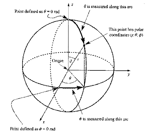
To describe such an expanded 3D Structure, it was first necessary to define an adequate set of 3D coordinates. The best known of these is 3D Cartesian axis system which define the direction and extent of atomic of Structure or Behaviour properties on three open-ended axes (x, y, z). However, most stable atomic Structure and Behaviour properties are based on the continuous rotation of electrons in uncertain but closed pathways around the nucleus, forming a sphreical shape in space.
To describe any property of a system, it is easiest to use a coordinate whose "axes" have the same shape as the system itself. Thus to describe these spherical atomic properties, a set of closed "Spherical Polar" 3D coordinates are usually used, consisting of the set of closed "Spherical Polar" 3D coordinates, shown in Figure (1) Their spherical form mkaes them mathematically "covariant" with the closed spherical Structure of the atom, that is the coordinate axes vary the same way as the spherical shape shape of the atom being described.
Thesespherical coordinates use the radius r, to describe the extent of radial displacement of a property from the nucleus in any direction, the azimuthal angle, theta, to show the extent and specific direction of any angular displacement down from the vertical direction and the horizontal rotation angle, phi to show the extent and specific direction of any angular displacement in the horizontal plane around this vertical axis.
Figure
1 Spherical
polar coordinates, related to Cartesian coordinates The Standing Wave Analogy for Atomic Structure
Schroedinger used these spherical polar coordinates to express all of the Structural and Behavioural properties of atoms.
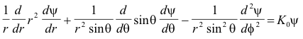
The dependence of the wave function ψ on the angular coordinates θ and φ can be separated from its dependence on the radius r to give two independent equations;
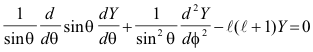
and
giving the two independent parts of the wavefunction, Y(θ, φ) and R(r)
The infinite number of 3D patterns traced out by the movements of bound but uncertain electrons are called their "wave functions". When these wave functions are squared and integrated over space and time, they define static patterns of averaged electron positions, called "probability distributions".
The shapes of these static patterns depend on the interplay of all of the forces acting on the bound electrons within the closed system. Acting together, these forces restrict the "allowed" patterns of motion into specific "standing waves" in which all motions are repeated endlessly through fixed positions. This restricted repetitive motion is familiar in musical instruments. Plucking a 1D string or hitting a 2D drum at different points, as shown in Figure (2), produces different "Linear Harmonics" or "Circular Harmonics" of motion respectively.
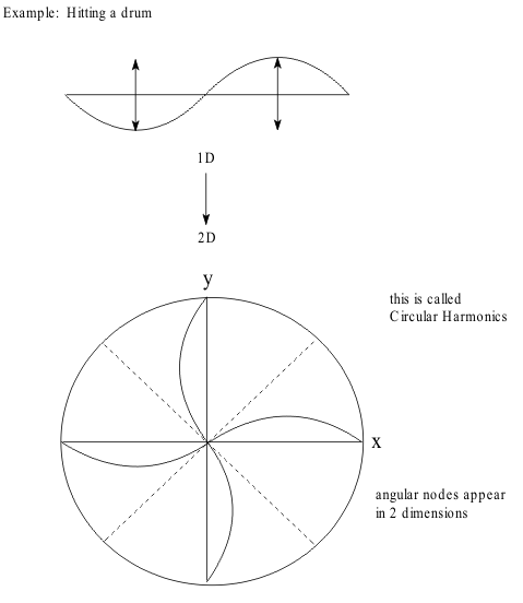 Figure 2 1D
Linear and 2D Circular Angular Overtones called Harmonics
Figure 2 1D
Linear and 2D Circular Angular Overtones called HarmonicsThese Harmonics are patterns of vibrational motion, which define the dynamic “Structure” of the vibrating object. During vibration, the different areas or volumes of the object move in opposite directions which are separated by positions of zero motion, called "nodes".The number of nodes defines the degree of the "overtone" which hasbeen stimulated and this degree is used to define the appropriate "quantum number", l
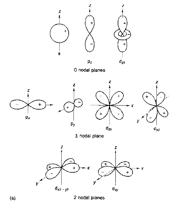 Figure 3 The Angular Nodal Planes of the 3D
Spheical Harmonics of Atoms, for l = 0, 1, 2
Figure 3 The Angular Nodal Planes of the 3D
Spheical Harmonics of Atoms, for l = 0, 1, 2The way in which each of these modes is stimulated, called its mechanical origin, is described in Table (1). Exploiting this musical analogy, Schrödinger used the mathematical functions called "Spherical Harmonics" to describe the shapes of these 3D standing waves of bound electron motion. Their individual shapes are represented by a spatial form of spherical polar coordinates. Since these patterns of angular momentum do not change with time, they actually create the stable "Structure" of the atom.
Table (1) The Mechanical Stimulation of Overtones of a Two-Dimensional Surface
|
Overtone |
Striking Position |
Number and Type of Nodes |
Quantum No. |
|
Zeroth |
Middle |
None |
= 0 |
|
First |
Half way to edge |
1 angular node |
= 1 |
|
Second |
Quarter way to edge |
2 angular or (1 angular +1 radial node) |
= 2 |
To emphasize this, Schrödinger called these standing spherical wave patterns the "orbitals" of the atom. Next, he adapted the the statistical mechanical definition of the average density of classical moving matter to define the quantum mechanical probability of finding the bound electron at any point in space as the square of its pattern of motion. Finally, since the whole electron must be found in all space, he defined the "normalization" of the integral to be 1.0.
Momentum Definitions for a Theoretical Periodic Table
However, these wave functions equally represent the "angular momentum", I of the bound electrons which form each standing wave. To identify the directions and speeds of these electrons, with the all of the certainty allowed by Heisenberg's Uncertainty Principle, the wave functions are written in an alternativemomentum form of Spherical Polar coordinates. This alternative set of identifying labels (n, l, m), is called the electronic Quantum Numbers.
The principal quantum number, n, defines the energy of the electron at its average radius. Then, for each n there is a nested set of (n-1) azimuthal quantum numbers, which define the changes in average energy when the orbit is "tipped" away from the vertical axis of rotation (the azimuth) of the angular momentum space to each allowed rotation angle. For each, a nested set of (2+1) magnetic quantum numbers, m, ( +1, 0, -1 ), which define the changes in energy when the orbit "precesses" around this vertical axis at the angles allowed by an external magnetic field.
Radial Wave functions
Both Schrodinger's equation (2.2) and the theoretical enrgies for H atoms imply that all orbitals labelled "ns" correspond to an increasing number of radial overtones. The shape of the (2s) orbital is shown in Figure (4 a and b). These show a radial node, at which the probability of finding the electron goes to zero in an infinitely thin spherical suface at a fixed radius from the nucleus. The node is shown in cross section in Figure 4a and as a Probability profile in figure 4b.
The cross sectional illustration shows the node as a circle at a fixed radius.
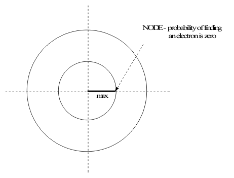 Figure 4 The Cross Section of the 2s Orbital
Showing its Radial Node
Figure 4 The Cross Section of the 2s Orbital
Showing its Radial NodeThe probability profile shows the node as a point of zero electron density at the same distance from the nucleus of the atom.
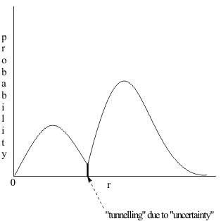 Figure 5 The Probability Profile of the 2s
Orbital
Figure 5 The Probability Profile of the 2s
Orbital