Group 4A; The Covalent Bonding Main Elements
Overall Relationships of Structures to Activities
The Elements of Group 4A again begin in the second row of the Periodic Table because the filling of the (1s)2 orbital of Helium completes the first row of the Table. All Group 4A Elements have electronic configurations [Rare Gas ](ns)2(np)2, with n from 0 to 7.
Spatial and Electronic Structures of the Elements
As in Groups 2A and 3A, the (ns)2 electrons can penetrate the core of filled p orbitals from all directions but as before, this core provides a shield with no defects which makes this valence pair of electrons unstable. However, this shielding is even more effective against the (np)2 electrons which can only penetrate to the nucleus from the two ends of its p lobe. Thus, in general, these (np)2 electrons are more easily removed than the (ns)2 electrons. However, in Carbon, the [(1s)2] core provides generally poor shielding and both types of valence electrons can easily penetrate through to the nucleus. Thus, the difference in their penetrating powers is not important. However the core becomes very effective down the Group to Tin and Lead, so the difference in penetration by their valence (ns)2and (np)2 electrons becomes much bigger.
The net effect of these shielding conditions is that the Effective Nuclear Charge ZEff, begins at moderate values in Carbon and decreases down the Group. This leads to a progressive increase in the atomic radius, representing the spatial aspect of atomic Structure of and a decrease in Hardness and Electronegativity, representing the electronic aspects of atomic Structure. The correlation of electronic configurations to spatial and electronic Structures is shown in Table 1
Table 1 Group 4A Correlation of Electron Configuration to Electronic Structure
| Element
Name |
Structural
Configuration
[core electrons] (valence electrons) |
r
nm |
η
kJ/M |
χ
kJ/M |
| Carbon | [(1s)2] (2s)2 ( 2p)2 | 0.17 | 487 | 605 |
| Silicon | [(1s)2(2s)2(2p)6] (3s)2 (3p)2 | 0.21 | 328 | 465 |
| Germanium | [(1s)2(2s)2(2p)6(3s)2(3p)6] (4s)2 (4p)2 | 0.2 | 318 | 445 |
| Tin | [(1s)2(2s)2(2p)6(3s)2(3p)6(4s)2(3d)10(4p)6](5s)2(5p)2 | 0.22 | 280 | 425 |
| Lead | [(1s)2(2s)2(2p)6(3s)2(3p)6(4s)2(3d)10(4p)6(5s)2
(4d)10(5p)6] (6s)2 (6p)2 |
0.2 | 270 | 430 |
Oxidation of the Elements
As in Group 3A, the Hardness and Electronegativity of Group 4A Elements begin at moderate values in Carbon and decrease down the Group to Lead. In these Group trends, the Electronegativity of most Group 4A Elements is still less than that for some nonmetallic Elements but usually more than that of most metallic Elements. Thus, in reactions between Group 4A Elements and these more Electronegative nonmetals, Pauling’s Electroneutrality Rule again predicts that, to minimize the energy of the whole system, the Group 4A atoms would lose electrons from either or both of the (ns)2 and (np)2 orbitals to the nonmetallic Element. This “oxidizes” the Group 4A Element to a stable cation of Oxidation Number +II or +IV and reduces the nonmetallic Element. For the +IV cations, the Structural parameters are given in Table 2.
Table 2 Electronic Structures of Stable Group 4A Oxidation Number +IV
| Stable
ON |
Configuration
[Core](valence) |
r
nm |
η
kJ/M |
(106)α
(nm3)M/kJ |
χ
kJ/M |
Π (10-4)
kJ/Mnm |
| C +IV | [ He ](2s)0 (2p)0 | 0.015 | 15800 | 0.0006 | 22000 | 145 |
| Si +IV | [ Ne ](3s)0 (3p)0 | 0.025 | 5880 | 0.007 | 10200 | 40.8 |
| Ge +IV | [ Ar ](4s)0 (4p)0 | 0.04 | 2300 | 0.083 | 6750 | 16.9 |
| Sn +IV | [ Kr ](5s)0 (5p)0 | 0.07 | 1520 | 0.68 | 5450 | 7.8 |
| Pb +IV | [ Xe ](6s)0 (6p)0 | 0.078 | 1280 | 1.11 | 5350 | 6.9 |
As with Group 3A Elements, when the nonmetallic Element acquires the valence electrons of the Group 4A atom, it is “reduced” to a stable anion. In reaction with the Halogens, X2 ;
M + 2X2 ⇒ MX4 (1)
The resulting anion can then form any type of chemical bond to the Group 4A cation.
As was first observed in Group 3A, with the formation of stable compounds of Tl +I, these Elements have high enough intermediate Ionization Potentials that they exhibit stable +II Oxidation Numbers in many compounds. Their Structural parameter values are given in Table 3.
Table 3 Electronic Structures of Stable Group 4A Oxidation Number +II
| Stable
ON |
Configuration
[Core](valence) |
r
nm |
η
kJ/M |
(106)α
(nm3)M/kJ |
χ
kJ/M |
Π (10-4)
kJ/Mnm |
| C +II | [ He ](2s)2(2p)0 | - | - | - | - | - |
| Si +II | [ Ne ](3s)2(3p)0 | - | - | - | - | - |
| Ge +II | [ Ar ](4s)2(4p)0 | 0.07 | 880 | 1.17 | 2400 | 3.45 |
| Sn +II | [ Kr ](5s)2(5p)0 | 0.09 | 770 | 2.85 | 2175 | 2.42 |
| Pb +II | [ Xe ](6s)2(6p)0 | 0.12 | 815 | 6.35 | 2265 | 1.89 |
Also, as first observed in a few Boride derivatives from Group 3A, the lightest of these Group 4A Elements have such high Electronegativities, that they are capable of forming the negative, stable Oxidation Numbers -II and -IV, corresponding to the configurations [Core](ns)2(np)4 and [Core](ns)2(np)6 in many compounds. However, there are no empirical Electron Affinity data for these isolated anions which would allow any calculation of the Mulliken Structural parameters.
Reduction of the Elements
In contrast to this oxidation chemistry, in reactions between these Elements and the less Electronegative metals, Pauling’s Electroneutrality Rule predicts that, to minimize the energy of the whole system, the Group 4A atoms would gain electrons into their unfilled (np)2 orbital from the metallic atom. This reduces the Group 4A Element to a stable anion of Oxidation Number -II or -IV and oxidizes the metallic Element to a stable cation. For example, in reaction with the Alkali Metals, M, the Group 4A Element, Y would react to form ;
4M + X ⇒ M4X (2)
The resulting cation can then form any type of chemical bond to the Group 4A anion, to form such compounds as Li4C, called “lithium carbide”.
Bonding Structures of Group 4A Elements
In general, the type of [ M-X ] bond, ionic, donor covalent or covalent, depends on the relative polarizing powers Π and polarizabilities α of the two Elements forming the bond pair. However, in the specific case of Group 4A, these Structural parameters have values intermediate between those found in Elements at the beginnings and ends of Periods. This makes the Group 4A Elements “electronically amphoteric” so that they usually achieve charge satisfaction by covalent sharing rather than by ionic exchange of electron pairs. In spite of this, it is still very useful to identify the Oxidation Numbers of Group 4A Elements in their compounds in order to describe how electron pairs are rearranged during reactions. The range of Oxidation Numbers is again limited by the Structures of the previous and the next rare gas respectively, giving an upper limit of +IV and a lower limit of -IV for atoms in this Group. However, since these atoms are usually covalently bound within the Structures of compounds, their Oxidation Numbers cannot be assigned from direct experimental measurement of the their charges. Instead, the Numbers must be assigned theoretically on the basis of the relative Electronegativities of the atoms in the bond, as they were defined in the Rules for Stable Oxidation Numbers;
1 The Stable Oxidation Number (SON) of the most Electronegative Element, Fluorine is -I
2 The SON of the least Electronegative Element, Cesium is -I.
3 The SON of intermediate Electronegativity Elements is positive, (+N) when bonded to Elements of higher Electronegativity and negative, (-N) when bonded to Elements of lower Electronegativity.
4 The sum of all Oxidation Numbers of all atoms in the compound equals the external, total charge on the compound, ( = 0 for a neutral molecule or = (+N) in molecular ions ).
Carbon Compounds
When these Rules are applied to carbon compounds, they assign SON values over the entire a range from the lower to upper rare gas limits. The electronic configuration of Group 4A shows that the valence, representing the completion of the Octet of the next rare gas atom, is always 4. Thus, all one-carbon compounds have the molecular formula X4C and the final SON Rule for them becomes;
4(SON)X + 1(SON)C = 0 (3a)
hence, 1(SON)C = 0 - 4(SON)X (3b)
This expression can be used to identify the value of (SON)C in compounds with Elements of higher, similar to and lower Electronegativities than Carbon. Examples are given in Table 4
Table 4 SON Values for Carbon in X4C Compounds
| Compound | χX | (SON)X | (SON)C |
| Li4C | 230 | +I | -IV |
| H4 | 625 | +I | -IV |
| CF4 | !000 | -I | +IV |
Alkanes
Alkanes are the “saturated” hydrocarbons in which the C atom has four single covalent bonds to either H atoms as shown for methane in Figure 1 or another C atom..
The Structure at each C atom is “tetrahedral” with a bond angle of 109.9o. When the C atom is bound to other C atoms or”catenated”, normal, branched or cyclic chain compounds are formed, which are named systematically. This naming system uses the roots “meth”, “eth”, “prop” and “but” for chains of 1 to 4 Carbons but follows a numerical system for all longer chains. Side chains are identified by their numerical starting point on the longest chain. Cyclic alkanes are named by the largest ring.
Reduced and Oxidized Alkane Derivatives
When alkanes are reduced with the alkali metals, they form covalently bonded metal derivatives, with (C-M) single bonds. This is illustrated in Figure 2 by the derivative n-pentyl lithium.
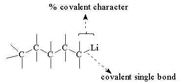
In simple terms, the SON of carbon is not altered by this reduction but its chemical reactivity is completely different from the initial alkane, pentane.
On the other hand, if an alkane like CH4 is oxidized, a series of progressively hydroxylated compounds is produced up to the ultimate oxidized product, CO2. These oxidation reactions increase the SON of carbon in steps of +II, increasing its Electronegativity above that for Hydrogen at the second step. As each H2O is released, dehydrated product is formed, as shown in the Section on Group 3A. Similar processes occur when the alkanes are oxidized by Nitrogen, Phosphorus and Sulfur, producing similar sequences of derivatives, shown in Figure 3.
Thus, in both cases, the SON assignments shown in Table 5 give a qualitative explanation the Structure and Activities of these derivatized alkanes but cannot predict details like the altered reactivity of the reduced derivatives or the spontaneous rearrangements of the oxidized derivatives.
Table 5 SON Values for Carbon in Hydroxylated Hydrocarbon Compounds
| SON | -IV | -II | 0 | +II | +IV |
| Initial Formula | H4C | H3COH | H2C(OH)2 | HC(OH)3 | C(OH)4 |
| Final Formula | H4C | H3COH | H2CO | HCO2H | CO2 |
| Compound Name | Methane | Methanol | Methanal | Methanoic Acid | Carbonic Acid |
Silicon Compounds
In the silicon atom, the 3p valence electrons are shielded away from the nucleus by the filled (2p)6 core. This shield destabilizes electrons in the 3p valence shell very strongly because it has the same shape of the 3p valence orbital. It also makes all single bonds from the 3p orbitals very unstable. The types of known single bonded Silicon compounds are given in Table 6.
Table 6 SON Values for Silicon in X4Si Compounds
| Compound | χX | (SON)X | (SON)C |
| Ba2Si | 250 | +I | -IV |
| SiH4 | 625 | +I | -IV |
| SiF4 | !000 | -I | +IV |
Reduced and Oxidized Silane Derivatives
Like methane, silane, SiH4 may be reduced by alkali metals to produce silicides of Lithium, Potassium and Barium. However, the instability of the 3p electrons forces the silicon away from isolated anions into a polymeric Structure of tetrahedral Si4 units.
Also, like methane, silane may be oxidized by the Electronegative Halogens to produce tetrahedral SiX4 derivatives which are again covalent molecules. However, its reactions with O2 pass through all the steps without producing stable intermediate products, to give the final oxide ;
SiH4 (g) + 2O2 ® SiO2 (s) + 2H2O (4)
where SiO2 is a hexagonal crystalline ionic solid, rather than a covalent molecular gas like CO2. This difference between carbon and silicon chemistry is entirely caused by the instability of the 3p valence electrons. The shielding by the filled (2p)6 core increases the radius of the 3p orbital so much that silicon atoms cannot approach the oxygen atoms closely enough to achieve the pπ-pπ overlap needed for stable (Si=O) double bonds. Instead the oxygen atoms are force to make two single bonds to different silicon atoms. This creates a lattice of (Si-O) single bonds and results in formation of the solid product known as quartz.
In the heavier Elements, Germanium, Tin and Lead, the shielding of the np orbital increases further. This increases their radii and stabilizes the +II Oxidation Number. Consequently, these Elements display no double bonding and their compounds become more ionic.
Structures and Activities of Group 4A Compounds
These Group 4A compounds have a very wide range of bond strengths which are essentially independent of their equally wide range of bond types. As well the reactivities of these compounds range from very slow “Inert” to very fast, “Labile”again independent of bond strengths. Thus, the Structures and Activities of these compounds cannot be described or predicted by the Lewis Acid-Base model. That model was only designed to describe the predominantly polar bonding in the previous Groups and was not concerned with the speed of their reactions because most of them proceed to equilibrium as fast as substances can diffuse. Thus, for these compounds of Group 4A and the later p-block Elements, a better model of Structure and Activity is needed. This new model can be derived from their most basic Activity, their ability to resist change, usually called their “Stability” which depends on two variable aspects of their relationship to the external environment;
1 The time-independent question of whether they could change in their environment.
2 The time-dependent question of how fast they would change in existing conditions.
Empirical Evidence of Group 4A Stabilities
1 The Possibility of Change
To decide if a compound could change in a particular environment, its internal energy is compared to the energy available in the external environment. This difference in energy was defined by Willard Gibbs in 1918 as the “Free Energy” ΔG of the compound with respect to its environment. In this definition, he formally assigned energy flowing “endergonically” into a compound with a positive sign and energy flowing “exergonically” out with a negative sign. However, the First Law of Thermodynamics says that energy must always flow from high to low potential. Thus, only those compounds with negative Free Energies with respect to the environment could react spontaneously. Then, some or all of the negative Free Energy in the “Reagent” is released to the environment and a different “Product” would be formed. The energy released represents the spontaneity of the reaction. It can be measured experimentally by Calorimetry, but for a reaction ;
A + B - C + D (5)
Reagents Products
it is calculated as the difference between Free Energies of Formation of reagents and products ;
DG0 Reaction = Σ DG0Products - Σ DG0Reagents (6)
This calculation was first defined by G. N. Hess in 1840 and is therefore known as Hess’ Law.
However, to set up data bases of the Free Energies of Formation of all known chemical compounds under all conditions is just as difficult as making all the direct measurements. In the liquid or solid environments common in chemical operations, the Free Energies of Formation and Reaction are essentially independent of pressure but they do depend strongly on both the concentrations of reagents and products and on the system temperature. Thus, a single set of standard conditions known as Standard Temperature (293.15 K) and Pressure (101.35 kPa) has been defined by international agreement and is maintained in trustworthy facilities. The agreements were made through the International Union of Pure and Applied Chemistry (IUPAC) and the facilities are maintained in many counties by independent organizations such as the National Research Council of Canada. The Standard Free Energies measured at these STP conditions are denoted as ΔG0.
Concentration Dependence
The concentration dependence of the Free Energy of Reaction can be plotted as a function of reaction yield, on a “Reaction Coordinate” Q . The Free Energies at 0% and 100%, correspond respectively to the Free Energies of Formation of pure reagents and products from their Elements.
Between these limits, Hess’ Law defines a straight line called the “Theoretical Reaction Path”. Depending on its sign, the total Free Energy of Reaction ΔG0 Reaction becomes linearly more negative for exergonic spontaneous reactions or less negative for endergonic non-spontaneous reactions, as the yield goes from 0 to 100% along the Reaction Coordinate. However, from equation (5), the yield, Q can also be expressed as the ratio of the concentrations of products to reagents. Then the constant slope, K of the Hess’ Law line can be written as ;
which, can be integrated to give the log form of this correlation as ;
This dependence of ΔG Reaction on the ratio of product to reagent concentrations makes its value too dependent on the physical reaction conditions to be used as an identifier of the chemical reaction. However, since ln(1.0) = 0, the ratio term can be eliminated by setting all concentrations in (8.7b) to a Standard condition of 1.0 Molar. Then ΔG Reaction only depends on the constant of integration, which is independent of concentration conditions. It can therefore be used as a unique characteristic of each reaction and defined as the “Standard Free Energy of Reaction”, ΔG0Reaction at STP.
Thermodynamics therefore shows that a fully balanced chemical equation must not only describe the balancing of the quantities of materials as moles of reagents and products in a reaction but must equally account for the total energy balance. Essentially this defines a balancing of the “moles of heat”exchanged with the environment during the reaction. Thus in a typical chemical reaction such as the complete oxidation of an alkane ;
CH4 + 2O2 ⇔ CO2 + 2H2O (8)
it is necessary to define the Free Energy absorbed or released, in kJ/M.
Temperature Dependence
However, after removal of its concentration dependence, the value of ΔGReaction still depends on temperature. To define this dependence, Gibbs adapted the usual physical definition of the total energy of any system to identify Free Energy as the sum of potential and kinetic factors. However, he recognized that these two factors had completely different dependencies on temperature. In most chemical systems, the potential energy is determined by the Coulombic forces holding atoms together. These forces are only weakly temperature dependent and Gibbs defined their energy content as Enthalpy, with the symbol ΔHReaction . In contrast, the kinetic energy of the system is determined by the amount of free movement of atoms which is directly temperature dependent. However, by factoring out this direct temperature dependence, Gibbs was able to define a term another weakly temperature dependent term called Entropy, with the symbol ΔSReaction . These factorization are summarized in Table 7
Table 7 Factorization of Total Energy
| Energy Definitions | Energy Factorization | ||||
| Physical |
Total Energy |
= |
Potential Energy | + | Kinetic Energy |
| Thermodynamic | Free Energy | = | Enthalpy | - | Temperature x Entropy |
| Symbolic | Δ G | = | Δ H | - | T ⊗ Δ S |
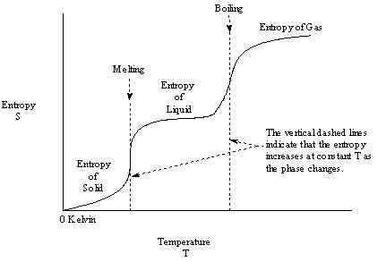
As with the total Free Energy each of these factored terms is again defined as a difference from a Standard calibrated value. Since Enthalpy originates essentially in the potential energy stored in bonded Structures of chemical substances, there are no unique physical condition in which the potential energy goes to zero. Thus, in order to quantitate ΔHReaction it is necessary, as with ΔG Reaction to set the arbitrary Standard Zero for Enthalpy in the pure Elements at STP. On the other hand, the kinetic energy inside the internal Structure of a pure solid Element does go to zero at 0 K.
Thus, it is possible to measure Standard Molar Entropies of the Elements at STP by integrating the Entropy accumulated during warming up from 0 K, as shown in Figure 5.
Thus, each of these three terms must be calibrated to Standard conditions of the Elements. Since each thermodynamic term refers to a different aspect of the stabilities of chemical substances, separate standards are defined and maintained for each of them. For the pure Elements, the conditions are listed in Table 8.
Table 8 Standard Definitions and Conditions of Thermodynamic Properties of Elements
| Thermodynamic Term | Value
kJ/M |
Temperature
K |
Pressure
kPa |
| ΔG0 | 0 | 298.15 | 101.35 |
| DH0 | 0 | 298.15 | 101.35 |
| DS0form | 0 | 0 | 101.35 |
The single criterion for the spontaneity of chemical reactions based on Free Energy must now be expanded into sets of criteria created by all of the combinations of signs and magnitudes of Enthalpy, Temperature and Entropy. The four basic conditions of reaction spontaneity determined by the possible combinations of the signs of Enthalpy and Entropy are collected in Table 9.
Table 9 Correlation of Thermodynamic Term Signs to Reaction Spontaneity
| Spontaneity | Sign of Thermodynamic Term | ||
| ΔG | ΔH | ΔS | |
| Spontaneous | - | - | + |
| Non-Spontaneous | + | + | - |
| Spontaneous if T is low or DS is small | - | + | + |
| Spontaneous if T is high or DS is large | - | + | + |
2 The Speed of Possible Changes
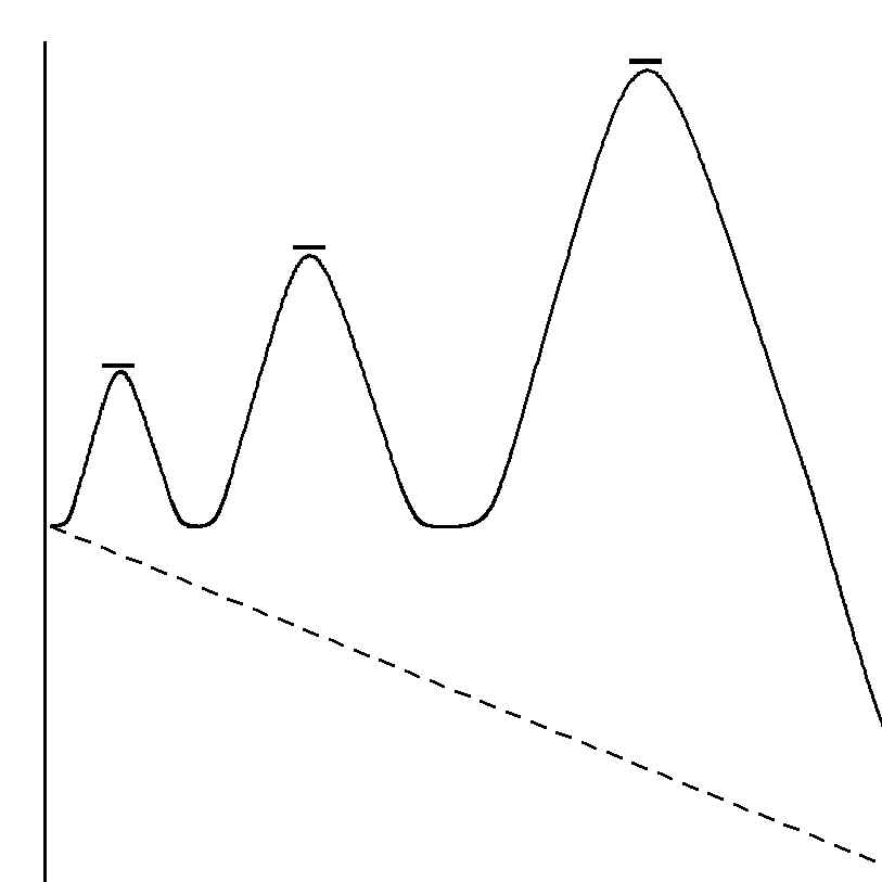
However, determining that a reaction is thermodynamically spontaneous does not guarantee that it will achieve 100% yield in experimental conditions, indeed, it may not start at all. Moreover, if it does start, the rate of reaction can vary from extremely fast, going to completion in nanoseconds to extremely slow, with completion requiring millions of years. Neither of these extremes of reaction Activity can be described using the simple Theoretical Reaction Path, in Figure 4.
Labile Reaction Paths
In the very fast reactions, the high rate occurs because, at the start of the reaction, there is an immediate and very large negative change in Free Energy. In fact, on these “Labile Reaction Paths” the change may so large that at some intermediate yield point Q on the Reaction Coordinate;
DG0 Reaction < Σ DG0Products (9a)
Thus, the “forward reaction” would only reach completion if the system could endergonically reacquire this ejected Free Energy back from the environment. Since this is forbidden by the Second Law, the only option for the forward reaction is to slow down until it is equal to the “back reaction”rate. At the Q value where this happens, Figure 5, a “true equilibrium” is established, where the forward and back reactions proceed at equal rates. For this reason, the Labile reaction paths are called “reversible”. Since both forward and backward reactions are sensitive to concentration, equation (6b), and to temperature, QEquilibrium alters with any such changes in the environment, following Le Chatelier’s Principle.
Inert Reaction Paths
In the very slow reactions, the low rate occurs because at the start of the reaction, there is an immediate and very large positive change in the Free Energy of Reaction. In fact, on these “Inert Reaction Paths” the change is always so large that, at a Q of 0% on the Reaction Coordinate;
DG0 Reaction > Σ DG0Products (9b)
Thus, the “forward reaction” cannot even start unless the system endergonically acquires this Free Energy from the environment. In principle, this is again forbidden by the Second Law and if all molecules in the reaction mixture behaved identically, no forward reaction would be possible
On the other hand, the energy could be supplied to some of the molecules without breaking the Second Law on average, if they had a range of behaviour. This actually does happen because, at any temperature, T, the molecules of the reagents are randomly organized, so that their kinetic energies range widely around the average value.
Therefore, a small population of molecules always has enough energy to proceed up to the top of the endergonic, non-spontaneous “Activation Barrier”of the Reaction Path to the “meta-equilibrium” at a characteristic yield QMetaEquilibrium. At this Q, these at any T molecules are both thermodynamically Unstable and kinetically Labile because their forward and back reactions are equally spontaneous and impose no additional Activation barriers.
This point is called the “Transition State” of the reaction. If the back reaction starts, the reaction mixture returns to pure reagents. If the forward reaction starts, it converts completely to products without stopping at any intermediate point. Therefore, these Inert Paths are called “irreversible” and are not altered by environmental conditions.
Thus, to decide the rate at which the compound would actually change, the potential energy“barrier” to change within the compound must be compared to the kinetic energy level of the environment. In simple terms, if enough kinetic energy is supplied to the compound as heat or light, it will start reacting. The role of this difference in energy between the potential barrier and the external kinetic energy as the single factor regulating the rate of any spontaneous reaction was first recognized by Svante Arrhenius in 1888.
The barrier energy is now called the “Free Energy of Activation” of the reaction, DG*Activation, The Reaction Rate Constants, k, corresponding to these Activation Free Energy barriers are defined by the Arrhenius relationship ;
DG*Activation =- RT [ln k] (10)
where R is the gas constant (8.314 J/K/M ) and T is the Standard Temperature, (298.15 K ).
If ΔG*Activation is large and the reaction very slow, the compound is described as “kinetically Inert”. If ΔG*Activation is small and the reaction fast, the compound is described as “kinetically Labile”
Reaction Kinetics
The value of DG*Activation, can therefore be determined by calculating or measuring the speed of each spontaneous reaction at different temperatures The technique used to measure these speeds is called Reaction Kinetics. In liquid and solid media, it is clear form equation (7b) and Figure 6 that these speeds again depend on both the reagent concentrations and the system temperature.
Concentration Dependence
The speed of any Inert reaction at constant temperature is defined by the rate of loss of one of the reagents such as A. It always depends on the rate constant k and could depend on the concentration of one or more reagents ;
Rate = k [A]A [B]B (11)
where the superscripts A and B represent order of the reaction in each reagent. The overall order of the reaction is then defined as the sum of the reagent orders ;
Order Reaction = Σ [ A + B + ... ] (12)
Often the rate of loss of reagents depends on the concentration of one reagent such as [A] ;
![]()
then, the reaction is “first order” in [A] and [A] decreases exponentially with time. On the other hand, if the reaction rate depends on the concentrations of both of the reagents, [A] and [B] ;
![]()
then the reaction is first order in each reagent and by adding these orders together is “second order” and overall. As the result, [A] decreases quadratically with time. However, it is often difficult to recognize the difference between these two curve shapes, shown in Figure 7, when plotting the usual imperfect and uncertain experimental data..
To make it easier to recognize the order of reactions, the data are linearized. For first order reactions, the data are replotted by first rearranging (13) to separate the variables so that ;
![]()
then as before, the rate equation can be integrated to convert the exponential form to a log giving a plot of ln [A] versus time; between the time limits from 0 to ∝ ;
![]()
This linearized form is plotted in Figure 8, giving a straight line with a negative slope.
For the second order reactions, the data are linearized by separation of variables:which is plotted in Figure 9,
giving a straight line with a positive slope.
Temperature Dependence
In the rate data plots, the effect of temperature appears as an increase in the initial slope because the reagent is consumed faster at higher temperatures, as shown in Figure 10.
increasing rate constants k from these curves can then be plotted against the temperature. Experimentally, Arrhenius found that this was an exponential relationship with the equation ;
![]()
which could again be linearized by separating variables and integrating ;
which gives the linear Arrhenius plot of ln k against 1/T at constant [A] shown in Figure 11.
However, since Arrhenius defined the relationship of rate constant k to the Free Energy of Activation from equation (10) as;
ΔG*Activation = - RT ( ln k ) (18a)
and the Gibbs factorization of Free Energy to Enthalpy and Entropy from Table 7 is ;
DG*Activation = DH*Activation - T ⊗ DS*Activation (18b)
then, by substitution;
- R [ln k] = T DH*Activation - DS*Activation (18c)
which is the equation of a line with slope -ΔH* and intercept ΔS*. Thus, the Arrhenius equation plays the same role in kinetics that Hess’ equation plays in thermodynamics, by defining the Enthalpy, Entropy and Free Energy of Activation for the Transition State.
Classification of Stabilities
Thus, to describe the overall stability of a compound, A, both the Spontaneity and the Rate Constant of all of its possible reactions in its particular environment with the general balanced form;
A + B ⇒ C + D (19)
must be identified and assessed by either direct experimental measurements or by estimation of the Free Energies of Reaction and Activation from Tables of Standardized data. Then, its stability against all possible processes of change can be classified into one of the four Stability Categories shown in Table 10, where “kT” represents the kinetic energy available from the environment.
Table 10 Stability Categories
| Thermodynamic | ||
DG0Reaction (-) ⇒ Exergonic ⇒ Unstable |
DG0Reaction (+) ⇒ Endergonic ⇒ Stable | |
| Kinetic | ||
DG*Reaction < kT ⇒ Labile |
DG*Reaction > kT ⇒ Inert | |
Chemical Interpretations of Stability
Following the 800 year-old philosophy of finding the simplest explanation, expressed in "Occam’s Razor", the purpose of Chemistry has always been to find the simplest adequate way to explain and predict these Stabilities. Thus, the first models described Stabilities simply by assigning atomic Oxidation Numbers and estimating bond strengths and types from Polarizing Powers and Polarizabilities. While these were adequate for compounds of alkali metals, these Classical models could not explain the Structural differences between gaseous CO2 and solid SiO2 or Activity differences like the Inertia of methane, compared to the Lability of silane in air.
These new requirements showed that an adequate model of Stability had to combine the static properties of the Stable Group IV compounds with the dynamic properties of the Labile compounds. This type of theory is called a “Reaction Mechanism”model and its necessary static and dynamic properties are defined together on the Reaction Pathway, Figure 4. On these Pathways the static property of the reaction is defined as its spontaneity. It is quantitated by Hess’ Law as the Free Energy of Reaction between the Free Energies of Formation of the pure reagents and products.
This Free Energy can be factored into sums of potential and kinetic energy contributions, following Table 7. Each factored term continues to obeys Hess’ Law of static properties;
ΔH0Reaction = Σ ΔH0Products - ΣΔH0Reagents (20a)
and
ΔS0Reaction = ΣΔS0Products - ΣΔS0Reagents (20b)
On the same Pathway, the dynamic property of the reaction is defined as its lability. It is quantitated by Arrhenius’ Law as the Free Energy of Activation as its rate. This is quantitated as a difference of initial and “Transition State” functions and calculated from the magnitude of the Free Energy of Activation between the Free Energies of formation of the pure reagents and the “Reaction Complex”. Following the previous relationship from Gibb’s definitions in Table 7, this Free Energy is then factored, if needed, into the sums of potential and kinetic energy contributions defined by equation (18)
Thus, it was essential to find a model which would be able to describe the static and dynamic aspects of both the spontaneity and the labilty of all Group IV compounds. The first consequence of this requirement was that any model used to describe spontaneity from the Reaction Free Energy of these compounds must incorporate the Structural fact that their bond strengths SB, which range from very weak to very strong are completely independent of their bond types TB which range from ionic to covalent. The second consequence was that the description of lability in the new model must incorporate the Activity fact that the reaction spontaneities of Group 4A compounds range from endergonic to exergonic but are completely independent of their reaction rates, which range from essentially zero to the diffusion rate.
Quantal Interpretation of Reaction Spontaneity
In the Lewis models used to describe the properties of the compounds of earlier Groups of Elements, two static properties of atoms are used to recognize these two aspects of bonding. These properties are essentially two arbitrarily independent factors of Free Energy, called the Hardness and Electronegativity or equivalently, the Polarizing Power and Polarizability of reacting atoms. In contrast, in all Quantal models, this dual property of bonds is recognized by defining one static and one dynamic property of valence electrons.
These properties are essentially two independent factors which follow Gibb’s factorization of Free Energy into Enthalpy and Entropy in equation (20a,b). The static property, which represents the Reaction Enthalpy, is interpreted Quantally as the difference in potential energy of the valence electrons on the separate atoms. On each atom, this potential energy is usually defined as the “Valence State Ionization Potential”. These VSIPs can be quantitated by either the Semi-empirical or Theoretical (often called ab initio “from the beginning”) methods. However, the change in Reaction Enthalpy, ΔH0Reaction from reagents to products depends not only on these separate atom VSIPs but also on any changes in the number and geometry of bonds during reaction. Thus, in Quantal models, ΔH0Reaction must include the energy changes due to any Structural differences from reagents to products.
The dynamic property formally represents the change in Entropic energy TΔSReaction of the valence electrons as the bonds change. Since Entropy represents the disorder of systems, this change in Entropy during reaction formally defines the change in the freedom of motion of the valence electrons. Essentially this represents the change in their kinetic energy. This is described Quantally as an overlap of the valence orbitals The simplest case to illustrate this overlap condition is the H2 molecule. Before overlap, the configuration of each H atom is (1s)1. As the atoms approach, the overlap of valence orbitals is described as a “Linear Combination of Atomic Orbitals”.
The type of LCAO Molecular Orbital formed a t the time of contact depends on whether the radial wave function of each 1s atomic orbital is either expanding. If both AOs are expanding or contracting at the same time, their overlap is “In-Phase”, making their interference constructive and their wave function amplitudes add together in the overlap region. This type of LCAO MO increases the probability that electrons would occupy this region. This decreases the order of the valence electrons because they can now occupy a larger common volume with more freedom of motion. This increases their Entropy and hence stabilizes the MO with respect to the separate AOs. As a result this MO is called a “Bonding MO”, as shown in Figure 12.
Since this particular Bonding MO is constructed from the (ns) AO's of H atoms, it is identified as an nsσ (using the Greek equivalent of s as σ ) MO. On the other hand, if one of the AO's is expanding while the other is contracting, their overlap is “out-of-phase”, making their interference destructive and their wave function amplitudes subtract from each other in the overlap region, This LCAO MO eliminates the probability that electrons could occupy this region and this decrease in common volume remove some freedom of motion of the electrons. This destabilizes the MO with respect to the AO's and it is called an “Antibonding MO”, as shown in Figure 13.
Since this Antibonding MO is constructed from the (ns) AO's of H atoms, it is identified as an nsσ* MO. The plane of zero electron density between the 1s orbitals of this MO is a "node". With this Quantal interpretation, the spontaneity of reactions can now be defined and predicted as the most probable rearrangement of valence electrons during reactions.
Quantitation of Structures
Most organic compounds are so complicated that only the Semi-empirical methods of estimating the VSIPs and overlaps of their valence orbitals are practical. In these methods, the HOAO energy is defined by the first Ionization Potential of the isolated Donor atom, IPD and the negative values on the vertical axes of an “Energy Diagram” to represent the stabilities of bound electrons on infinitely separated atoms. In "homonuclear diatomic molecules" the HOAO's of the atoms are then "stabi;lized", during in-phase σ overlap into the Bonding MO.. Similarly, the LUAO's are destabilized by out-of-phase σ* overlap into the Antibonding MO. The energy Level Diagram for the homonuclear molecule, H2 shown in Figure 14 illustrates this way of describing the purely covalent bonding of these molecules.
In "heteronuclear diatomic molecules" the in-phase σ overlap of the filled HOAO of the Donor with the empty LUAO of the Acceptor atom forms the Bonding Molecular Orbital. The out-of-phase σ* overlap of these orbitals again forms the Antibonding Molecular Orbital.
Thus. in these molecules, the Bonding Molecular Orbital is "predominantly" stabilized by the Ionization Potential of the HOAO of the Donor atom IPD "modified" by the Electron Affinity of the Acceptor atom EAA. Likewise, the destabilization of the Antibonding Molecular Orbital is "dominated" by the Electron Affinity of the Acceptor atom EAA, and "modified" by the Ionization Potential of the HOAO of the Donor atom IPD..
To quantitate the energies of both the Bonding and Antibonding Molecular Orbitals, the Average Valence Orbital Energy is defined by the Donor HOAO and Acceptor LUAO energies;
Then, the "ionic contribution" to the total stabilization of the heteronuclear bond is defined by the difference between this average Energy and the IPD ;
and the "covalent contribution" is defined by the stabilization beyond IPD due to the overlap, S, of the Acceptor LUAO with the Donor HOAO. This is often quantitated as the approximation,
which was first suggested as a simple approximation by M. Wolfsberg and L. Helmholtz in 1952. Many more accurate (but more complicated) approximations have been tried since then.
The advantage of this approximation is that it only needs simple calculations with readily available data to describe any type of bonding from covalent to ionic, at any strength from weak to strong. The total bond stabilization energy is then the sum of the Ionic and Covalent energy stabilizations, (11a,b);
However, rather than using the raw atomic data, the calculation is more often done with the equivalent chemical data of atomic Hardness and Electronegativity to correlate this LCAO MO model directly to the Lewis Acid-Base description. To do this, the energy term used to estimate both the Ionic and Covalent contributions is restated as follows ;
then substituted into (11c) to give the total energy or Strength of the bond, SB ;
The necessary Hardness and Electronegativity data can be taken directly from the Tables given for each Group of the Periodic Table. In the special case when these energies equal, the Energy Level Diagram simplifies to show only the σ Bonding and σ* Antibonding orbitals of a purely covalent, homonuclear diatomic molecule like H2. Using only Hardness and Electronegativity in semi-empirical approximations of Classical models or initial AO energies in Quantal models only represents the electronic part of the atomic Structures of the bonding atoms.
This is corrected in the Classical Lewis Acid-Base model by incorporating the effects of radial and angular aspects of atomic Structure into the Polarizing Power and Polarizability of separate atoms. In contrast, in Quantal models, these effects are condensed into their common overlap term, [1+S]. Thus, the two models do include the same information, but the final bond Structure of a Classical model is described as a distortion of the separate atom properties, defined before bond formation due to mutual contact, while in a Quantal LCAO MO model, it is described as a phased interaction of common properties, defined after bond formation, due to their interpenetrating overlap.
Each type of model has its own particular advantages. In Classical models such as Valence Bond Theory and Valence State Electron Pair Repulsion Theory, the atoms are described as charged, soft bodies which can attract each other and adapt the shapes of their separate electron densities to increase their joint stability. This description has the advantage that the semi-empirical estimation of atomic Polarizing Powers and the Polarizabilities and the Classical electric dipole calculation of bond energies are very simple. It has the disadvantage that it only describes the bonding energy and leaves Antibonding MOs undefined. In contrast, in any Quantal model such as LCAO MO theory, atoms are described as charged, penetrable bodies which can attract each other but now share their electrons according to the phases of their orbital overlaps to increase or decrease their joint stabilities.
This description has the advantage of giving both simple expressions, Equation (14) and illustrations, Figure 8, of all Bonding and Antibonding orbitals. It has the disadvantage that all these overlap values, called the “overlap integrals”, must be calculated separately for each valence orbital. This problem was so severe that, as early as 1949, Mulliken and coworkers in Chicago were publishing large tables of the necessary overlap integrals in order to help chemists estimate the nature of bonds in covalent or polar covalent molecules. In modern calculations, the theoretical models still concentrate on this problem.
Quantal Definition and Evaluation of Bond Strength and Bond Type
Both Classical and Quantal models show that bond strength, SB and bond type, TB are independent molecular properties. Classical model define these properties on the basis of two atomic parameters defined before bond formation. The simplest models use atomic Hardness and Electronegativity but the more refined models use atomic Polarizing Power and Polarizability.
In both cases, SB is readily calculated but defining TB generally requires a separate calculation of the redistributed charge after bond formation. In contrast, the Quantal models provide the values of both bond properties in one calculation. The value of the SB is found directly from the sum of the ionic and covalent energies, from Equation (14) and TB is found directly from the ratio of these same energies ;
It can also be stated as a ratio in terms of the of the Lewis Acid-Base parameters of Hardness and Electronegativity by substituting the definition from equation (22a,b ) to give the ratio;
Thus, while SB and TB are both derived from equations (15a,b), they express the two different properties of bonds in proper units; SB in energy units and TB without any units, since it is a ratio. The basic conclusion from these definitions is that the magnitudes of SB and TB are not related and therefore bond strength, SB cannot be either interpreted or predicted from bond type, TB.
However, in defining the energy in equation (15a), the opposing thermodynamic directions of the endergonic Ionization Potential and the exergonic Electron Affinity result in a reversal of sign between the terms for Hardness and Electronegativity. Thus, the Quantal definition of SB, shows that the bond is most stable when the term depending on the Hardnesses vanishes. However, since this term depends on the difference in Hardnesses, it vanishes when they are equal, regardless of their magnitudes. This theoretical conclusion is strongly supported by the pioneering work on the stabilities of Lewis Acid-Base complexes by Frederick Basolo and Ralph Pearson, who showed that the most stable complexes were always formed between bond partners of equal Hardness, regardless of their Electronegativities.
Quantal Bond Order
While σ and σ* Molecular Orbitals are the only types relevant in the Hydrogen molecule, the energy and overlap definitions can be extended to describe the involvement of the (np) AOs of p-block Elements in the bonding Structures of homonuclear diatomic molecules. The overlap AOs gives rise to two more MO geometries. The first forms from the end-to-end overlap of the
(np)z AOs along the direction of the bond.
Since this MO is directed along the bond, like sσ and sσ* AOs, it becomes a pσ Bonding or pσ* Antibonding Molecular Orbital, depending on its phase of these relationship. The second type of MO forms from the side-to-side overlap of the (np)xy AOs. This generates MOs with electron density directed across the bond. To denote this“lateral” geometry, it is called a pπ (the Greek equivalent of p) Bonding or a pπ* Antibonding MO, as shown in Figure (16), depending again on its phase relationship.
All of these types of Molecular Orbitals obey the Pauli and Aufbau Principles which govern the electron occupancy of Atomic Orbitals. Applying the same Principles to these Molecular Orbitals, a Molecular Configuration can be defined, equivalent to an Atomic configuration.
Thus, the electronic Structure of the C2 molecule would be described by an MO Configuration written as; [(1sσ)2(1sσ*)2(2sσ)2(2sσ*)2](2pσ)2(2pπ)2. The MO configurations of all the other homonuclear-nuclear diatomics are defined in the same way. In the N2 molecule, the completed MO configuration fills the Bonding and Antibonding MOs formed from overlapping AOs, such as (1sσ)2(1sσ*)2, as shown in Figure 17.
In general, these MOs are self-cancelling pairs and filling the Antibonding MO cancels the energy stabilization achieved by filling the Bonding MO. Thus the net bonding effect of these filled pairs is zero. As a result, these filled pairs are called the Core of the MO configuration and have very little influence on either the Structure or the Activities of any molecule. To complete this energy level diagram description of the MO Structure of a homonuclear diatomic molecule, the available electrons are inserted into the MOs following the Pauli and Aufbau Principles, as shown in the general heteronuclear energy level diagram in Figure 18.
With the heteronuclear diatomic molecules, the shapes of the stable orbitals stay the same but the Ionization Potentials of the AOs of the different atoms are different. The stabilisation of the Bonding MOs and the destabilisation of the Antibonding MOs are again plotted between the axes to represent the changes resulting from increasing overlap as the atoms approach from infinite separation. To complete the description of this type of MO Structure, the available electrons are inserted in the MOs according to the Pauli and Aufbau Principles, as shown for a typical heteronuclear diatomic molecule in Figure 18.
These examples illustrate the concept called “Bond Order” which is defined in all Quantal MO models but is unknown in the Classical models. It is quantitated as the difference between the number of stabilized and destabilized valence electron pairs ;
which, for the molecule in Figure 12 becomes ;
= [1 + 2] - [0.5} = 2.5
Thus, Bond Order concerns only the actual numbers of Bonding and Antibonding pairs, regardless of their strength or type.
Quantal Interpretation of Reaction Inertia
Just as for the static properties of Group IV compounds, any model of their Activities must equally be able to explain how the rates of their reactions can range from very slow to very fast but be completely independent of the strength of the reacting bond. In the Lewis model, this distinction was not made because essentially all reactions of compounds of the earlier groups of Elements proceed directly to an equilibrium on the Reaction Pathway. In contrast, the compounds of the Group IV Elements are often Inert and react very slowly, in spite of being placed in conditions of spontaneous reaction. This situation is represented on the Reaction Pathway Figure (5.4), shown again in Figure 19, as the Free Energy of Activation, ΔG*Activation , between the Free Energies of Formation of the reagents and the Transition State complex.
Figure 19 Definitions of Reaction and Activation Free Energies
As before, the Quantal models can be used again in these “transitional” situations to interpret the Free Energy of Activation as an excitation energy of the valence electrons of the participating reagents. Then, following Hess’ Law, this excitation energy is factored in equation (18) into the Activation Enthalpy and the Activation Entropy.
The Activation Enthalpy is then interpreted as the potential energy excitation of the valence electrons by static Coulombic Repulsion between reagents. This potential energy is estimated as the “Transition State Ionization Potential”. The Activation Entropy is interpreted in a parallel way as the kinetic excitation due to the dynamic Phase Interference of these valence electrons and is estimated as the “Transition State Covalent Energy”. This energy contribution comes from the tunnelling of the valence electrons between the reacting orbitals during their transient overlap in the Transition State shown in Figure 19..
Therefore, just as in the quantitation of Reaction Spontaneity in terms of the Reaction Free Energy, the quantitation of Reaction Lability requires an evaluation of both the static Enthalpic and the dynamic Entropic factors in the Activation Free Energy. This means that a Quantal Reaction Mechanism model of the Transition State is needed. The physical factors in these models are defined according to the dependence of reaction rates on all experimental conditions. One of these experimentally important conditions is the concentrations of reagents as was given above in equation (11);
Rate = k [A]A [B]B (11)
In the models, this experimental dependence on reagent concentration is interpreted as a theoretical dependence on the distance between reagent molecules. This is because, to achieve a Transition State, these models assume that reagent molecules must first find each other by random collisions. The inverse dependence of reaction rates on reagent concentrations occurs because, as the concentrations of the reagent molecules increase, they get closer together and collide more often.
If this random collision process was the only factor determining the reaction rates, then the order coefficients, A and B, would be the same as the stoichiometry coefficients, a and b, of the balanced form of the reaction, first given above as equation (5) ;
aA + bB ⇒ cC + dD (28)
Reagents Products
This correlation may be true for very fast spontaneous labile Reaction Pathways but experimental evidence almost always shows that there is no connection between reaction rates and Stoichiometric coefficients on spontaneous inert Reaction Pathways. Instead, from equation (11), the Rate of this type of reaction depends on the order coefficients as powers of the reagent concentrations ;
Rate = k [A]A [B]B (30)
where each of these order coefficients may have any value 0, 1, 2, .. . This disconnection shows that there must be a second important factor determining how reagent molecules behave as they move along these spontaneous inert Reaction Pathways, towards their Transition State complexes.
The nature of this second factor is shown by the direct dependence of these rates on temperature in the Arrhenius equation, (8.17a,b). Since reaction temperature essentially defines the kinetic energy distribution of the reagent molecules, Figure 20,
This second factor is defined in Reaction Mechanism models as the speed of movement of the reagents at the collision. On spontaneous inert Pathways, only a very small number of collisions actually lead to reaction. However, as the temperature increases, the % of molecules with enough speed, shown as (T) in Figure 20, to collide hard enough to get over the reaction Activation Energy barrier increases exponentially, following Arrhenius’ equation. This leads to a common “Rule of thumb that by raising TReaction by 10̊C the rate of reaction will double.
However, even when the collisions are hard enough to provide the necessary Enthalpic energy for the reaction, they are usually not oriented properly for the reaction to go forwards to products. Thus, the Activation Free Energy barrier also depends on the Entropic order of reagents in the Transition State complex.
The more complicated the shapes of the reagents, the less likely they are to be in the right positions for reaction during collisions. In particular, this Entropic problem of requiring only the correct reaction orientations would make biochemical processes far too slow to support life as we know it. The only way to increase reaction rates above this random collision rate is to add a reaction site
As shown in Figure 21, this can reduce the barrier at constant temperature by either reducing the Enthalpic requirement of a severe enough collision, when the site is called a catalyst or, as is the case for most biochemical reactions, by reducing the Entropic requirement through organizing the reagents into the necessary reaction geometry, when it is called an enzyme.
Mechanisms of Reactions
From these interpretations of spontaneity and inertia, all Reaction Mechanism models start describing reactions by using the order coefficients in the Arrhenius equation to define how many molecules of each reagent are needed to set up the Transition State. Since these are different from the Stoichiometric coefficients, these models identify this complex as the highest energy point on the inert Reaction Pathway.
However, the Stoichiometric coefficients show that all of the reagents must be used in their proper proportions, so there must be other “complexes” before or after the complex defined by the rate coefficients when all the other necessary changes occur. Therefore most models represent the complete Reaction Pathway as a multi-step process, shown in Figure 22, of which only the slowest step, called the “Rate-Determining Step”, can be observed in the reaction kinetics measurements.
Thus only the behaviour of reagent molecules which participate in the slowest step can be described by any model. The behaviour of the remaining molecules must be found from other types of evidence.
Thus, Reaction Mechanism models all start by factoring DG*Activation with Gibbs’ definition;
ΔG*Activation = ΔH*Activation - TΔS*Activation Table 7
despite the fact that it is a property of a transient species and not independent of time as a true State Function should be.
In this “State”, most models interpret DH*Activation as the potential energy needed to distort reagent structures enough to break old bonds. As shown on the methane molecule in Figure 23, this could involve any combination of stretching or bending of a (C-H) bond until it breaks.
The same models interpret TΔS*Activation as the energy needed to orient the methane molecule so that the bond-breaking process can actually occur. At very high TReaction the (C-H) bond could have enough vibration energy to break by itself. At his limit, the Transition State complex is simply this excited methane molecule. This means that the Rate-Determining Step is the rate of breaking the (C-H) bond in each molecule and that the rate of this “Unimolecular” reaction would be first order in methane concentration, [CH4]1. Since eventually some other species, R would replace the missing H atom, the Mechanism is called a “Substitution, Nucleophyllic, Unimolecular”, abbreviated as SN1.
At lower TReaction , the (C-H) bonds would not be vibrating enough to break by themselves but could break if attacked by a second reagent, “R”. Then the Reaction Mechanism theories must provide two different types of information. One is the distribution of electrical charge around the Structures of the reagents and the other is the availability of valence orbitals where bonds can be broken and formed. The charge distribution is needed to describe the way that the reagents will be attracted to each other from a distance. Since these attraction forces can act on separated reagents, this is often called the “long range effect”. The valence orbital availability is needed to describe the covalent interactions of reagents in the Transition State complex which allow the electrons to tunnel from old bonds around to new bonds. Since this tunnelling can only occur in overlapped orbitals, it is often called the “short range effect”.
As shown in Figure 23, the reagent R could either attack at the end of a (C-H) bond or it could enter a triangular “face” of the tetrahedral Structure. If R was negatively charged, the long range effect would be an end-on attack at the positive H atom, with SON (+I). Since R is attacking the positive part of methane, the Mechanism is described as a “Substitution, Nucleophyllic (positive-loving), Bimolecular”process, abbreviated to SN2.
The Transition State complex would be the union of methane with R along the temporary, short-range {C-H-R} bond. The Rate-Determining Step would be the over-stretching the original (C-H) bond, to the breaking point, while temporary valence orbital overlap allowed electrons to tunnel from the original (C-H) bond to the new (C-R) bond. The rate of this “Bimolecular” reaction would be first order in both methane concentration, [CH4]1 and reagent concentration, [R]1, making the reaction second order overall.
On the other hand, if R were positively charged the long range effect would be a face-on attack at the negatively charged carbon atom, with SON (-IV). Since R is attacking the negative part of methane, the Mechanism is described as a “Substitution, Electrophyllic (negative-loving), Bimolecular”process, abbreviated to SE2. The Transition State complex would be the union of methane with R along the temporary short range {C–R} bond.
In this case, the Rate-Determining Step would be over-bending of the original (C-H) bond, again to its breaking point, while temporary valence orbital overlap again allowed electrons to tunnel from the original (C-H) bond to the new (C-R) bond. Thus, the rate of this totally different type of “Bimolecular”reaction would again be first order in methane concentration, [CH4]1 and first order in reagent concentration, [R]1, making the reaction second order overall.
Quantal Models of Reaction Mechanisms
The existence of these three totally different Mechanisms, SN1, SN2 and SE2 shows that a very clear theory is needed to discriminate between their Transition States and to predict which of them would dominate the inert Reaction Pathway in any given set of reaction conditions. In the SN1 Mechanism, the Quantal model must simply identify the weakest bond to predict which bond would break in the Unimolecular Transition State. This can be done by the LCAO MO method.
However, in SN2 and SE2 Mechanisms, the Quantal model must describe the rearrangements of bonds in the Bimolecular Transition State. This can be done by an extension of the LCAO MO method. Just as the AOs which could overlap were linearly combined to construct the MOs of stable compounds, any of the reagent MOs which could physically overlap can be linearly combined to construct the transient MOs of Transition State complexes, in a “Frontier Orbital” method. The first step in applying this model is to recognize when reagent MOs can overlap. Then the second step is calculating the extent of overlap to find how fast the electrons can tunnel to the new bond.
To recognize when reagent MOs can overlap, two factors need to be considered. The first is the long range effect. The Coulombic forces between molecules define whether any two reagents will attract or repel and, if the attract, how they will line up with each other. The second factor is the short range effect. In the Transition State geometry set up by these long range forces, the short range effect determines if there are any allowed overlaps of the Frontier Orbitals. Just as in the LCAO MO models, the short range effect is based on the phase relationship between the Frontier Orbitals. In-phase Frontier Orbitals are allowed to overlap into transient bonds while out-of-phase Orbitals repel by forming transient antibonds. For the organic compounds of Group IV, this basic criterion was refined into a set of rules by R. B. Woodward and R. Hoffman in 1965. Once the LCAO MOs of any two reagents are known, the “Woodward-Hoffman Rules” can be used to predict whether they could possibly react on any one of the Reaction Mechanism Pathways.
If the Reaction Mechanism is allowed by both the long and short range effects, the Rate of Reaction is determined by how long and how well the Frontier Orbitals can overlap. These factors are opposite functions of TReaction . At low TReaction , reagents collide slowly, maximizing overlap time, but they collide weakly, minimizing overlap extent. At high TReaction, these factors are reversed. Thus, the Reaction Rate will actually be fastest at an intermediate TReaction where the best compromise of duration and penetration is achieved. In practice, this optimal TReaction is usually much higher than the Standard Temperature, 298K, so the Reaction Rates of most inert reactions do increase exponentially with TReaction following Arrhenius’ Law. The high temperature limits are only important for gas phase reactions at TReaction values above 500K.
Once this geometrically allowed and energetically optimized Transition State overlap of Frontier Orbitals is achieved, the electrons can start to tunnel to their new regions of space to become the new bonds in the product molecules. The final question is are they pulled or pushed to these new positions ?
They can be pulled out of their old positions if they can release Free Energy by going from the old bond to a more stable new bond. This pull-type of “electron transfer” Oxidizes the old position and Reduces the new position. The process is usually called an “Oxidative Addition” reaction because the incoming reagent is added to the target reagent by oxidizing an old bond. Alternatively, the old electrons can be pushed out of their original position because Free Energy can be released by avoiding an antibond pair donated by the incoming reagent. This donation of an antibond pair Reduces the old position and Oxidizes the new position. The process is usually called a “Reductive Elimination” reaction because the incoming reagent eliminates the old bond on the target reagent by reducing its antibond.
Thus, it is now commonplace to use these Quantal Reaction Mechanism concepts routinely to explain or predict the products of organic reactions.